Performance Engineering Through Tyre Management | Pt. 2

Balance by Numbers

Part 1 showed how centre of mass position and lateral load transfer distribution shape the force demanded of each axle and, in turn, the energy entering the tyres.

These mechanisms help us understand balance, but “understeer” and “oversteer” remain qualitative descriptions. To tune balance systematically, we need to quantify it.

Finding Neutral

Imagine a car travelling straight at a steady speed while an external lateral force is applied somewhere along its wheelbase.

Applied near the front axle, it creates a yaw moment in one direction; near the rear, it creates a moment in the other. Between them lies a point at which the car develops lateral motion without the introduction of any yaw rate. In the linear single-track model, both axles then operate at the same slip angle.

This is the Neutral Steer Point (NSP).

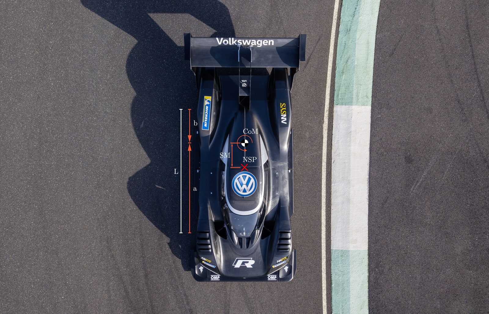
Mathematically, the NSP sits this distance behind the front axle centreline:

$$x_{\mathrm{NSP}} = \frac{L\,C_R}{C_F + C_R}$$

where L is the wheelbase, and C_F and C_R are the effective front and rear axle cornering stiffnesses. The greater an axle’s share of the car’s total cornering stiffness, the closer the NSP sits to that axle.

Notice that the CoM does not appear explicitly in this expression. The NSP divides the wheelbase in direct proportion to the effective cornering stiffness of each axle, much as an aerodynamic centre of pressure divides it in proportion to aerodynamic load. At a given operating condition, its position is set by the relative lateral force response of the two axles only.

The CoM is the centroid of the mass distribution, the NSP is the centroid of the axles’ lateral force response, and the CoP_Z is the centroid of the aerodynamic load.

Cornering stiffness of course varies with vertical load, tyre state, pressure and temperature, and so the NSP moves continuously through a lap. It is a dynamic parameter rather than a fixed property of the car.

The CoM is the centroid of the mass distribution, the NSP is the centroid of the axles’ lateral force response and the CoP_Z is the centroid of the aerodynamic load. These three centroids interact to define the car’s balance.

Mind the Margin

So if the NSP is a measure of how much each axle contributes to total lateral force developed during a corner, what we’re interested in, then, is to understand how this manifests in dynamics.

This is defined by where the NSP sits relative to the centre of mass. That distance is the Static Margin, a term brought over to vehicles from aeronautical engineering:

$$\mathrm{SM} = x_{\mathrm{NSP}} - x_{\mathrm{CoM}}$$

For the car introduced in Part 1, L = 2.6 m and x_CoM = 1.56 m. Taking C_F = 2400 N/deg and C_R = 3000 N/deg gives x_NSP = +1.444 m and SM = −0.116 m (ahead of CoM).

Notice that cornering stiffness has not scaled in proportion to axle load. The rear carries 1.5 times the front’s vertical load but returns only 1.25 times its cornering stiffness. That is tyre load sensitivity, the same sublinearity we leaned on throughout Part 1.

To allow us to view this quantity in a useful way, and draw comparisons to other vehicles and platforms, we normalise it by wheelbase. This introduces the concept of the Stability Index (SI), a dimensionless number that means the same thing on a kart as it does on an LMP car.

$$\mathrm{SI} = \frac{\mathrm{SM}}{L}$$

Our car returns −0.044.

The Stability Index describes the position of the NSP relative to the CoM in a wheelbase-independent form. Its sign identifies an understeering or oversteering characteristic, while its magnitude tells us how far the car sits from neutral. It is a linear, steady-state measure of how the slip-angle requirements of the two axles diverge as lateral acceleration builds.

Under the sign convention used here, SI > 0 places the NSP behind the CoM. The front slip angle then grows faster than the rear, producing an understeering characteristic. Conversely, SI < 0 places the NSP ahead of the CoM — the rear slip angle grows faster, producing an oversteering characteristic. At SI = 0, the axles operate at equal slip angles.

This is not simply a rule of thumb. In steady-state cornering, lateral force and yaw moment equilibrium determine the force required from each axle. Dividing those forces by their respective cornering stiffnesses gives the required slip angles. Subtracting one from the other gives:

$$\alpha_F - \alpha_R = m\,a_y\,\mathrm{SI}\left(\frac{1}{C_F} + \frac{1}{C_R}\right)$$

For our example, the difference develops at −0.33° per g. At the 1.5g condition used in our comparison, the linear model gives front and rear slip angles of 2.45° and 2.94°, respectively:

$$\alpha_F-\alpha_R=-0.49^\circ$$

The negative result confirms that the rear axle requires the greater slip angle.

Know Your Limits

Two limitations are worth stating plainly. First, the Stability Index is built from cornering stiffness, which is the initial slope of the tyre’s lateral force vs slip angle curve. It tells us which axle’s slip angle develops more quickly, but not necessarily which will saturate first. Saturation is governed by peak force, which is related to cornering stiffness but remains a separate tyre characteristic.

Second, SI describes only the sideslip-induced stiffness of the car, not its complete lateral–yaw response.

When the vehicle develops sideslip, the tyres generate a yaw moment. The Static Margin determines whether that moment restores alignment or pushes the car further away:

$$N_\beta=\mathrm{SM}(C_F+C_R)$$

Here, N_β is the yaw stiffness: the change in yaw moment produced by a change in sideslip.

For a given wheelbase and total cornering stiffness, its sign follows SI and its strength scales with the magnitude. Put simply, the sign tells us which way the car tends; the magnitude tells us how hard it tries.

A small positive SI produces gentle self-correction. A larger positive SI aligns the vehicle more strongly with its direction of travel. Negative SI reverses the effect: a small negative value gives a mild destabilising tendency, while a larger magnitude amplifies a disturbance more strongly.

A weathervane works in the same way. Place the effective response behind the pivot and it promotes alignment; move it ahead and it promotes divergence.

This relationship also appears at the steering wheel through steering gain. Put simply, steering gain describes how much vehicle response the driver receives for a given steering input. That response can be expressed as curvature, lateral acceleration or yaw rate; here, we use yaw-rate gain per degree of road wheel steer.

A high-gain car needs less steering to produce the same yaw rate. A low-gain car asks for more lock. Moving further into positive SI reduces steering gain, while moving towards neutral increases it. Move onto the negative side and the gain rises more aggressively.

More precisely, this is the car’s linear, steady-state yaw-rate gain. “Linear” refers to the assumed relationship between tyre force and slip angle. “Steady state” tells us that the response has settled onto a constant speed, radius and yaw rate. It does not describe how quickly the car gets there.

Two Cars, One Corner

The box-out puts numbers around this. It compares our car at SI = −0.044 with one at SI = +0.10, both travelling at 40 m/s through a 108.7 m radius corner and generating 1.5g. All steering and slip-angle values are outputs of the linear, steady-state model; they are not predictions of tyre behaviour at peak grip.

Two cars, one corner

40 m/s · 1.5 g · 108.7 m radius · equal total cornering stiffness

Quantity	Loose car	Stable car	Unit
Rear static-load fraction	0.60	0.60	–
Rear stiffness fraction	0.556	0.70	–
NSP behind front axle	1444	1820	mm
Stability Index (SI)	−0.044	+0.10	–
Static Margin (SM)	−116	+260	mm
Steer required	0.88	2.67	deg
Front slip angle	2.45	3.63	deg
Rear slip angle	2.94	2.34	deg
Yaw-rate gain	23.96	7.90	°/s per deg
Yaw stiffness (Nβ)	−624	+1404	N·m/deg
Yaw damping (Nr)	−227	−201	N·m/(deg/s)

The corner demands 1.5g and 21.1 °/s of yaw rate from both cars: if they travel through the same radius at the same speed, the motion is the same.

What changes is how much the driver must ask for. Our car needs 0.88° of steer, while the stable car needs 2.67°. Their yaw-rate gains are therefore 23.96 and 7.90 °/s per degree of steer. Viewed another way, our car produces more than three times the yaw response for the same input.

That extra stability is also paid for at the front tyre. The stable car needs 3.63° of front slip angle against 2.45° for our car - a ratio of 1.48; leading to approximately 48 per cent more sliding velocity. With the same front lateral-force requirement, that means approximately 48 per cent more front-tyre sliding power.

There is an easy trap here: higher steering gain does not necessarily mean a faster transient response.

Rotation generates a separate yaw-damping contribution:

$$N_r=-\frac{a^2C_F+b^2C_R}{V}$$

where a and b are the distances from the CoM to the front and rear axles.

The 1/V term matters. At twice the speed, the same yaw rate produces half the change in axle slip angles and therefore half the damping moment. Yaw stiffness has no equivalent speed term, so it becomes more influential relative to damping as speed rises.

Together with yaw inertia, these properties determine how quickly the response develops. A car with a small or negative margin may therefore feel settled in slow corners, where damping is stronger, but increasingly edgy as speed rises.

A Question of Character

Speed adds another layer. On the positive side, characteristic speed marks the point at which yaw-rate gain reaches its maximum before progressively reducing. A larger positive SI brings that speed lower. On the negative side, gain continues to increase until the car reaches its critical speed. Increasing the negative magnitude brings that limit closer to the operating range.

At SI = 0, the Static Margin contributes no spring-like self-correction, although yaw damping remains. The car is neutral rather than inherently unstable, but there is no positive margin to absorb changes in tyre condition, fuel load, aerodynamic balance or vehicle state.

It’s worth being clear about what that margin is actually for. The fastest car is not automatically the one with the largest positive SI, or one balanced precisely at zero.

Performance wants the force capacity of each axle to be well matched to what the corner demands, so neither end reaches its limit while the other leaves grip unused. SI does not tell us whether that has been achieved because it describes the linear response of the tyres rather than their peak capacity.

The fastest car is not automatically the one with the largest positive Stability Index, or one balanced precisely at zero.

What a positive margin buys is robustness. Balance moves as fuel burns off, tyres degrade unevenly and aerodynamic load migrates with speed and ride height. Carrying some margin helps keep the car on the stable side of neutral as those conditions change. Carry too much and the price is lower yaw-rate gain, more front slip and a car that asks more of its front tyres.

Pulling the Levers

The useful thing about SI is that it can be written as two simple fractions:

$$\mathrm{SI} = k_R - m_R$$

where:

$$m_R = \frac{x_{\mathrm{CoM}}}{L} = \frac{a}{L} \qquad \text{and} \qquad k_R = \frac{C_R}{C_F + C_R}$$

In other words, SI is the rear axle’s share of total cornering stiffness minus the rear static load fraction. Understeer requires the rear axle to contribute a greater share of cornering stiffness than it carries of static load. Every setup lever that alters SI works by moving one or both of those numbers.

That gives us plenty to work with. Tyre size and pressure, wheel kinematics, longitudinal and lateral load transfer, aerodynamic balance and instantaneous vertical load can all alter the effective front-to-rear stiffness distribution. Fuel burn can move the mass fraction too.

Add front roll stiffness, for example, and more lateral load transfer passes through the front axle. Because tyre response is load-sensitive, the loaded tyre gains less cornering stiffness than the unloaded tyre loses. Effective front axle stiffness falls, the rear stiffness fraction rises and SI moves in the positive direction.

But it is not a free stability button. The same load sensitivity can reduce the front axle’s peak force capacity, while its smaller share of cornering stiffness requires it to operate at a greater slip angle. That can mean more front sliding power and more heat for the front tyres.

Larger rear tyres or a rearward shift in aerodynamic balance can also increase the rear stiffness share, arriving at a similar SI by a different route. The latter is particularly useful to hold onto: aerodynamic balance can alter the car’s handling without adding or moving any mass.

Live and Direct

How do we measure this at a circuit? It’s not straightforward to measure C_F and C_R directly, and most championships don’t allow the optical slip-angle sensors to do so cleanly. Instead, we infer the understeer gradient K from channels already available in the logger, which can get you remarkably close with some well-gated maths:

$$\delta = \frac{L\,r}{V} + K\,a_y$$

The first term is the kinematic steer required for the corner. Subtract it from the measured road-wheel steer and plot the result against lateral acceleration; the slope is K. Truly steady-state corners are scarce, but most circuits provide at least a few useful windows.

The same quantity can be written as:

$$K = \frac{W_f}{C_f} - \frac{W_r}{C_r}$$

For our car:

$$K = \frac{3924}{2400} - \frac{5886}{3000} = -0.327\ ^\circ/\text{g}$$

That is the same 0.33° per g rearward slip-angle divergence we found through SI. One result comes from vehicle data; the other comes from the position of the NSP. They are two views of the same balance characteristic.

This brings us back to tyre management. Slip angle is not itself energy, but it produces lateral sliding velocity. At small angles:

$$|V_s| \approx V\,|\alpha|$$

and the associated sliding power is approximately:

$$P_y \approx |F_y|\,V\,|\alpha|$$

This force–sliding-speed relationship is also used by Chindamo et al. (2021) to estimate tyre sliding energy from logged vehicle data.

At the same speed and axle force, the axle requiring the greater slip angle therefore generates more sliding power. SI does not single handedly decide which tyre degrades first; combined slip, load, compound, driving style and heat rejection all matter, but it shows where the linear balance of the car is asking for more tyre motion.

That is the Stability Index in review: a compact link between mass distribution, cornering stiffness, slip-angle balance, self-correction, yaw-rate gain and tyre energy. It is not a complete vehicle model, but it turns “the car feels loose” into something an engineer can quantify, tune and verify. Over a stint, that understanding can be the difference between arriving at the flag on a working set of tyres and nursing one axle home.

Combined Acceleration: Two Axles, One Envelope

So far, we have looked at how engineering shapes the car’s balance and the work demanded of each tyre. The car sets the size and shape of the envelope; the driver decides how that capability is spent.

Most readers will know the size and shape of the utilised friction envelope as the friction circle, although friction ellipse is more accurate because longitudinal and lateral capability are rarely equal. Trackside, this is the g-g plot.

At vehicle level, we can represent an idealised envelope by normalising each axis against its respective maximum:

$$\left(\frac{a_x}{a_{x,\max}}\right)^2 + \left(\frac{a_y}{a_{y,\max}}\right)^2 = 1$$

Rearranged, it tells you what remains available on one axis for a given demand on the other:

$$a_y = a_{y,\max}\sqrt{1 - \left(\frac{a_x}{a_{x,\max}}\right)^2}$$

The square root is where it becomes interesting. Using half of the available braking still leaves approximately 87 per cent of the lateral capability. Look at it the other way round: surrendering only 13 per cent of maximum cornering releases half of the braking capacity. At the diagonal, approximately 71 per cent of each, the marginal exchange becomes one-for-one.

This is why a progressive brake release can carry useful combined acceleration into a corner. As steering demand rises, braking demand falls, allowing the driver to follow the boundary instead of stepping abruptly from one axis to the other. Maximum trail braking is not the answer to every corner; the transition simply needs to be deliberate.

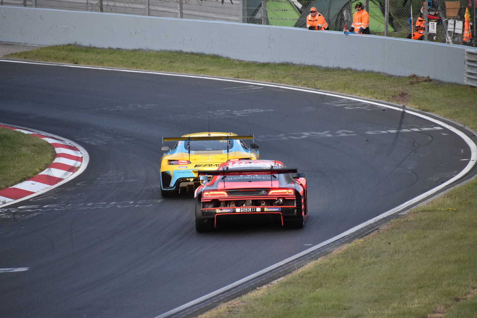
The envelope is not symmetrical either. Braking can use all four tyres, whereas traction is shared only by the driven wheels and further shaped by load transfer, power delivery and control strategy. The two halves of a real g-g plot therefore rarely match.

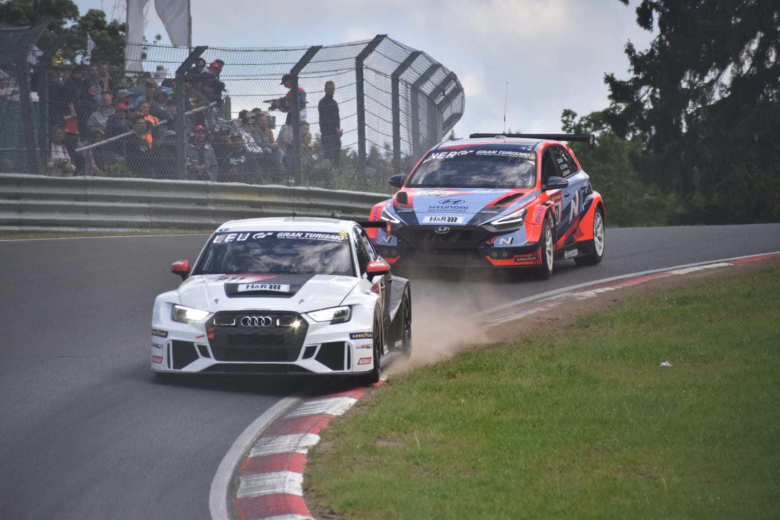
This matters immediately on a FWD car. Its front tyres steer, carry much of the braking demand and provide all the traction. The rear tyres have a much lighter energy workload, creating a strong front to rear imbalance.

TCR provides a particularly visible example of this. Rear tyres can struggle to reach their working temperature because comparatively little is being asked of them. After preparation runs, teams swap tyre sets front-to-rear (i.e. FL → RR, FR → RL, and vice versa), using the heat built at the busier front axle to bring the rear set into its operating window. That is tyre preparation built around an imbalance imposed by the drivetrain layout.

Twice the Price

In qualifying, the aim is generally to spend as much time near the useful boundary as the corner permits. In a race, operating slightly inside it may be deliberate: a little unused force can buy temperature control, tyre life or consistency, without a huge stint time hit. Beyond the peak, additional demand increases slip without producing more useful force and is a quick route to a world of pain.

Overdriving therefore charges twice: once in lost lap time and again in unnecessary tyre energy. The second cost may not become obvious until several laps later.

The useful question is not simply whether the driver is using all the available grip. It is how they move around the envelope, which tyres pay for it and whether that energy helps the stint or hurts it.

The engineer defines the envelope through setup, systems and tyre state. The driver decides how closely to follow it, where to leave a margin and when that margin is worth more than the immediate lap time. Combined acceleration is where those two halves meet, and both need to understand the other.

Across both parts of this article series, we have followed four levers: mass distribution, lateral load transfer distribution, Stability Index and combined acceleration. They may look like separate subjects, but each changes how force, slip and energy are distributed between four contact patches.

That is the useful shift in perspective. Understeer is not simply something a driver feels, and degradation is not simply something a tyre does. Both emerge from how the car and driver divide the work between the tyres, corner after corner. The setup defines the demand, the driver shapes it, and the tyre keeps the score.

The consequences are not always immediate. A poor energy distribution can hide within a single lap, then reveal itself as temperatures rise and grip falls across a stint. Tyre management is not simply the art of asking the tyres to do less. It is ensuring that the work asked of them buys lap time without borrowing too heavily from the laps still to come.

The setup defines the demand, the driver shapes it, and the tyre keeps the score.

A well-driven stint is an art form. A well set up car does not do the driver’s work for them; it provides the balance, confidence and usable envelope through which they can form a relationship with the machine. From there, car and driver work in symbiosis, responding lap by lap to what the tyres can give now and what they will need later.

A great stint is not extracted from a car by a driver. It is created between them. That is the beauty of racing.

Usual story: comments are welcome. Until the next one.

Download: the full stability model (Excel) — the complete two-car comparison, every input and output. Change any input and it recalculates.

Further reading

Chindamo, D., Gadola, M., Bonera, E. and Magri, P. (2021), ‘Sensitivity of Racing Tire Sliding Energy to Major Setup Changes: An Estimate Based on Standard Sensors’, Energies, 14(16), 5118. doi.org/10.3390/en14165118

Milliken, W.F. and Milliken, D.L. (1995), Race Car Vehicle Dynamics. SAE International — a comprehensive treatment of neutral steer, static margin, understeer gradient and vehicle stability.